A benefit of probabilistic surge forecasts - an example from Irene's impact on NYC

Here's a good site for surge predictions from SUNY Stonybrook.  The latest forecast for the Battery shows a good surge of 1-1.5 m above normal level in the early morning on Sunday.  You can see this forecast below where the dashed line is the expected forecast within a grey zone that represents the standard deviation of all the surge predictions at the Battery.  The red trace represents what the observed surge happens to be and the differences between observations and forecasts is represented in green.  Notice that the forecasts so far have been underestimating the observed water level most of the time.

The forecast surge height is one type of forecast but that doesn't tell how high the water will be relative to mean sea level.  Afterall, if the surge hits at low tide then the impact isn't as high.  So Stonybrook offers this second forecast timeseries superimposing the forecast tide on top of the surge and below is that forecast.

The timing appears bad if you don't want a flood.  The peak surge that you saw above happens to coincide with the morning high tide at the Battery yielding a water level 7 to 9 feet above mean low water.  This forecast is confirming why the New York City government placed mandatory evacuations of all low lying areas in their Zone A.  To see where Zone A exists, check out the city government site's interactive map at http://project.wnyc.org/news-maps/hurricane-zones/hurricane-zones.html

What is nice about these forecasts from Stonybrook is the grey zone of uncertainty.  It allows us to plan for reasonable worst case scenarios because forecasts have uncertainty.  But is the zone broad enough?  Will there be a surge higher than the grey zone?  The answer is quite possibly yes but the probability may be somewhat low.

Another site is available that shows the probability at which a surge is forecast to exceed some height, and also the surge heights as a function of probability.  I like the latter because it allows me to set my threshold probability for taking action and then I can see if the surge height exceeds my elevation.  Getting the forecast is easy.  Just go to http://www.nhc.noaa.gov/ and then click on the storm (Irene) and storm surge probabilities are listed above.  I choose the probability of a 5' surge and you can see the results below.  The forecast shows a 50% probability of a surge exceeding 5 feet in the New York harbour, even more around Staten Island.

  Of course the problem is how cautious do you want to be?  If you were sitting at 5 feet above the water would you move if the probability of you going under is at least 50%?  That's probably playing it a little too aggressive in my opinion.  Fortunately there's a website related to the one at  the NHC that allows you to dial your own probability.  Go to http://www.weather.gov/mdl/psurge/ and select the drop down menus until you find "20% exceedence height".  Now you see that the surge height forecasts are higher, 5 - 7 feet around the Battery to almost nine feet in western Staten Island.

So if you're a little more cautious, like me, perhaps you would dial in your personal probability threshold at 20% and you'll see that if you're below 5-7 feet above the water, you may want to move.  So to put it all together, here's what I'd do to decide for yourself if you need to move.  Note that I'm assuming you have no outside call for evacuation.

1.  Know my altitude above Mean Low Water
2.  Look at the tide forecasts closest to your site at http://tidesandcurrents.noaa.gov/gmap3/.  Click on the forecast point to get a menu and click on 'Tide Predictions'

3.  Determine the height above mean sea level (set at zero) for a set time.  Here I choose 8 am on Aug 28 and I get 5.5 feet.  That's high tide.  

4.  Then look at the probability of exceedence for at least 20%, preferably 10% from http://www.weather.gov/mdl/psurge.  We saw from above that 5-7 feet, so let's choose 7 feet.  

5.  Then add the value you got from 3 and 4.  In this forecast, 12 feet.

6.  Compare what you got from 5 with your altitude above mean low water.  If what you see from 5 is higher, then you make the decision to move.

Better yet, listen to the authorities because I do not espouse taking these steps above as the way to make a critical lifesaving decision when the authorities have so much more information at their disposal.  NYC produced a really nice evacuation map at http://project.wnyc.org/news-maps/hurricane-zones/hurricane-zones.html


BTW, the surge at the Chesapeake Bay Bridge was about four feet at 6 pm today.  That compared to a 20% exceedence of 5-7 feet.  So yes, you may have stayed dry if you were at least 8 feet above the high tide today which was 3.5 feet.  But why take chances?

The collapse of a stage at the Indiana State Fair 13 Aug 2011

Note:  I've added an addendum at the bottom of this post


Concert stage collapses from sudden wind gusts happen all to frequently and now we hear about another one occurring at the Indiana State Fair last night around 8:50 pm EDT.  The latest one was tragic with the loss of 5 people and multiple injuries, some of them life altering according to the Indianapolis Star.
To understand what happened, at about 8:50 pm, a gust front from a line of thunderstorms struck the stage just to the north of the main grandstand before the Sugarland concert was to begin.
This youtube video shows all the graphic detail of the stage collapse which unfortunately fell beyond the platform and into the VIP seating area full of people.




This tragedy was entirely preventable but a series of missteps aligned to put people in harms way. First, the stage was a 'house of cards', in other words, a flimsy metal scaffolding frame supporting a huge area of fabric facing the wind.   Second, it appears that people in charge of safety at the fair were determining when people should evacuate based on their uninformed interpretation of the meteorological data.  Mike Smith of WeatherData inc. eloquently described the issue with nonexperts serving the role as experts.  Needless to say this night proved how dangerous that can be.  Their hearts were nonetheless in the right direction as they began evacuation procedures.  This leads to a third problem.  Once they initiated evacuation procedures, not everyone was on the same page as the Daily Star reported that the WLHK program director addressed everyone with a mixed message, one that suggested to prepare for evacuation, the second that the show will go on.  Of course the very people closest to the stage would be the same ones least likely to take the first advice and most likely to stay on.

I first explore how strong the winds were likely to have been when the stage collapsed.  Well, that's not an easy question since there are no anemometers around the site.  But there are a few clues leading to a range of likely wind speeds.  One set of clues comes from what was not damaged.  I noticed a flagpole to the right and behind the stage that didn't blow over.  There were even tents nearby that remained.  Assuming a flagpole is similar in strength to a typical powerpole, typically 70 to 80 mph winds are required to initiate damage, sometimes less.  However there was no damage and so it's doubtful the wind exceeded 70-80 mph.  The same could apply to the many light standards around the fairgrounds in the video.  There were also no other reports of significant damage at the fairgrounds, a place full of large open span structures that could easily start to suffer damage at similar wind speeds (this is preliminary of course since I heard there was some minor nondescript damage scattered around the park).  I decided to take a stab at tracking identifiable plumes of dust that speed across in front of the stage platform.  The amount of time some of these plumes tracked across from one end of the platform to the other was about 1.6 to 2.5 seconds.  The stage measured 38 m long according to Google Earth (see figure 1) and that wind speed amounts to roughly 20-25 m/s or about 37-48 kts.

Figure 1.  A satellite view of the Indiana State Fairgrounds courtesy of Google Maps.  The inset shows the grandstand and the stage north of the dirt track.  The length of the stage platform is nearly 38 m and the wind direction was estimated from the WNW.

Could 37-48 kts be realistic?  Well, there is some supporting evidence.  The highest wind speed at the airport was 44 kts at 8:56 pm EDT.  In addition, to the south at the KIND WSR-88D, the highest winds at the radar site only reached to 40-45 kts (figure 2).  

Figure 2,  The KIND four panel display of reflectivity and velocity for 0056 UTC.  The half degree elevation shows up on the top row and the 2.4 deg elevation shows up on the bottom row.

Of course there are some reports that may indicate higher winds occurred in the vicinity.  One report occurred west of downtown about the same time as the stage collapse of a large tree blown down and an estimated wind speed of 70 mph attached.  Perhaps winds to 70 mph were there.  The other wind gust southwest of Indianapolis was considerably higher at a measured 77 mph. Power did go out around the town and by the next afternoon,  and about 1250 customers were still out of power.   Again, I'll wait and see if those winds occurred at the fairgrounds at various times but judging by the video, the wind speeds were considerably less and likely not even 50 kts when the stage collapsed.

figure 3,  A map showing the outline of the severe thunderstorm warning issued by the Indianapolis NWS forecast office, and the three local storm reports received during the course of the warning.

So the stage was set to put people at a high vulnerability level.  Certainly it appears this stage couldn't withstand winds any more than 45 kts and it's likely the stages that failed this year in Tulsa, OK Ottawa, ON, and last year in El Reno, OK also were similarly weak.  Too bad there was no communication as to the vulnerability of these stages from one set of event coordinators to another.

Given this vulnerability and the consequences of its failure,  the onus should be on the event handlers to provide an extra level weather awareness.  Unfortunately there was not since it appeared that the handlers were interpreting something for which they have no expertise.  In addition to in appropriate interpretation, the Indianapolis Star also reported that there was confusion as to when the threat would arrive.  The event handlers that Mike Smith mentioned,  waited till 8:45 pm to consider evacuation plans, four minutes before the stage collapse.  In addition, the Indianapolis Star quoted "According to a timeline issued today by Indiana State Police, at 8:49 p.m. -- about 25 minutes before the storm's forecasted arrival -- a strong gust of wind blew through the fairgrounds, toppling the stage setup onto the those closest to the stage.  Bursten said the early indication was that the "isolated significant wind gust" took authorities and event coordinators by surprise, since the storm itself was still about 30 minutes from arriving. They had been in contact with the National Weather Service for much of the evening." So it also appears that they were expecting a later arrival than what happened.   It's difficult to determine what the nature of state fair official's contact with the NWS had been but there is some evidence that there was some expectation that they had perhaps 25 minutes to prepare for severe weather.  What was the source of this misunderstanding?  

The NWS did issue a severe thunderstorm warning that covered the state fairgrounds and all of Indianapolis from when it was issued at 8:39 pm EDT.  As shown by the text below, the severe thunderstorm warning was issued as shown where an initial location of the threat was labeled and the entire area was covered in a polygon (figure 3 and 4).

AT 835 PM EDT...NATIONAL WEATHER SERVICE DOPPLER RADAR INDICATED A
  LINE OF SEVERE THUNDERSTORMS CAPABLE OF PRODUCING QUARTER SIZE
  HAIL...AND DAMAGING WINDS IN EXCESS OF 60 MPH.  THESE STORMS WERE
  LOCATED ALONG A LINE EXTENDING FROM 9 MILES NORTH OF ZIONSVILLE TO
  GREENCASTLE...AND MOVING EAST AT 25 MPH.

 The NWS marked the line of storms given the town landmarks from nine miles north of Zionsville to Greencastle (figure 4).  However, the text of the warning did not include the position of the gust front which was considerably further east.  

Figure 4 A map depicting the location of the severe thunderstorm warning and the 8:35 pm reflectivity.  Also the convective line (red) mentioned in the text of the warning is shown at the 8:35 pm position mentioned in the 8:39 pm severe thunderstorm warning.  The blue line marks the position of the gust front at 8:35 pm.

This is often the case that NWS meteorologists track the location of the heaviest, most likely severe, portions of the storm (s).  The problem is the way the event handlers may have interpreted the warning, and the location of the threat relative to the confines of the polygon.  The threat that was of the most interest to them should've been the gust front, not necessarily the worst of the severe weather that was located and tracked by the NWS forecasters.  The warning polygon gave the event handlers a lead time of 7-8 minutes before the gust front hit assuming a minute delay from warning issuance to their reception. That's when they should've taken action.  They would've needed all of that time considering that they had poor communication protocol amongst all the players in the warning dissemination, including the WLHK program director.

Large event handlers need a special relationship with expert meteorologists in order to help provide specific warning information.  Canned products are not enough because they don't provide the information that the handlers need nor does it give a tailored product to match the exposure of the event participants.  The severe thunderstorm warning from the NWS was fine but it didn't provide the handlers the timing of the gust front.   The handlers didn't know that they needed the timing of the gust front and so they were confused when the severe weather hit 20 minutes earlier than the actual line of heavy rain which the NWS was tracking.  Lacking knowledge, the handlers should've played it safe and evacuated early.  But the concert-goers, and program directors want to push the envelope and keep running the show till the last minute.  Wouldn't an event handler want a little more detailed information to help resolve these sometimes conflicting needs?

The concert stage was a flimsy structure where upon collapse, proved deadly.  It appears that not even severe thunderstorm threshold winds were needed to collapse the structure.  Thus it's entirely feasible that this tragedy could've happened without a severe thunderstorm warning.  When considering exposure level, everyone has a different threshold at which their safety may be compromised.  Consider figure 5 below that conceptually illustrates the varying thresholds of safety depending on the type of structure or situation for which someone may reside.  Each dot represents a situation where a person's safety is at high risk ranging from being in a small boat when the wind reaches 40 mph (special marine warning) all the way up to being inside a hospital or office building (140 mph).  These values vary from one situation to another but the point is made that each of us has a different exposure level and that official products do not account for this variety.  The event handlers need to know the exposure level of those in their charge and relay that to the meteorological consultants, in this case very low thresholds.  Then the consultants can use that information to make a better warning product.

Figure 5,  A conceptual diagram of exposure level vs. threat severity where personal safety can become compromised.  The threat severity happens to be wind speed.  Several examples are provided and compared relative to the severe thunderstorm wind speed threshold.

Typically when it comes to preserving life, the event handlers can choose to stoke a relationship with the NWS, either by an incident meteorologist (called IMET) physically present, on phone, or on chat.  Or a private sector company can be hired to be the consultant.  Certainly each has its advantages, the former is already paid for while the latter can devote more time and attention.  What should be communicated is what kind of exposure the people are subjected (e.g., under a flimsy stage, outside, in tents, in water), how much time he/she needs for evacuation, and any other special criteria.  The meteorologist can take these constraints and then give a forecast of when the relevant severe weather parameter is expected to strike.  The event handler may ask about the forecaster's confidence, and a reasonable answer should be given that conveys the truth.  Then the even handler can do what he/she has been trained to do.

Let's hope this message goes somewhere.


Addendum:

15 Aug 2011 - Now that a couple days have past, the questions arise as to whether or not the fair directors should've done more to protect the fair patrons.  This article at msnbc summarizes these questions quite nicely.  The questions fall into two camps, one related to who's overseeing the construction standards of temporary buildings, the other about who's responsible for executing a response to the warning of severe weather.  For the latter, I was intrigued to hear that an outdoor concert featuring the Indianapolis Symphony Orchestra at the Conner Prairie Amphitheater was canceled well before the storms hit.  Being that this venue was entirely outdoors with no protection, the concert directors had a plan, a source of expert weather advice, and a conservative attitude.  As a result, there would've been no news about their successful evacuation if it weren't for the tragedy at the fair.

As an aside, I hear some rather intriguing meteorologically-related theories as to why the stage collapsed.  They all have to do with some extreme local wind gust, even called a fluke that nobody could've forseen by the governor Mitch Daniels.   I hope this statement doesn't deflect the need to prevent future tragedies from collapsed stages.  This wind event was not a freak event never to show up again.    What is more likely is that the stage was such a house of cards that it fell where even tents stood less than 50 m away.  I tracked the plumes of dust across the stage platform and came up with rather modest winds of ~ 50 mph (~45 kts).  Perhaps my analysis was wrong and there were higher winds though I doubt I'm far off.   As the story on CBS confirms my thought, there was no freak anomalous wind that struck the stage, what was anomalous was the weakness of the stage.

The Great Sand Dunes NP 2011 on March 17-18

Daphne, and I decided to visit the Great Sand Dunes, NP in March 17-18 this year as part of our Colorado trip.  This park is one huge sandy playground and that's why I consider this place to be one of my favorites.   We started out at the visitor center to take a look at our plan by using this map.

An overhead view of the Great Sand Dunes where west is up.  I labeled the places we visited.

Here are some of the things we saw there.

Sand on the move

On the 17th, we were rewarded with a enough wind to see how the dunes come alive.  We thought we would have some fun on the first dunes past the dry bed of Medano Creek but instead we got to 'enjoy' blowing sand.

Since the first dunes were quite some distance away, we were thwarted from getting to them on this day.  Instead we played to the lee of a small bush of willows in the creek bottom and then on we went down a dirt road to the Medano Creek closer to the mountains where it was actually running (labeled 'Hike to Medano Creek' below).

Though it was still windy, this hike toward the creek was much less sand blown and we were afforded a much more pristine view of the sand. 

A view of the Great Sand Dunes from the end of the dirt road and the beginning of the sand 4WD trail.

Here, the Medano creek was flowing from the beginning of the spring snow melt season.  The creek helped blunt the worst impact of the blowing sand, though there was always some airborne grit.  Daphne was taking a picture of the creek but the constant pressure on the sand from her shoes liquified the sand and she began to sink.  We noticed that in the wet sand we couldn't stand still anywhere for any length of time.

Across the creek was a steep face of a sand dune.  The wind carried a continuous conveyor belt of sand depositing it on this lee face.   It didn't take long for a sand avalanche to commence.   Unlike the snow avalanche, this one was slow and subtle.  We tried to listen for the occasional singing sound the sand emits when a big sand avalanche occurs but in this wind, we couldn't hear anything so subtle.

Alamosa had reported wind gusts to 40 kts, judging by the load of sand in some of the gusts below, I'd say that's on the low end. 




Later in the evening after a meal in Alamosa, we returned to the sand dunes so I could shoot a sunset time lapse.  This time lapse below was taken at 12 fpm from the visitor center looking almost due north.  The wind was still strong and if you look carefully, you can see sand well above the dunes blowing east into the Sangre de Cristos.  Snow was also being blown off the top of Cleveland Peak to the north (see the map).  Throughout the time lapse, the orographic clouds formed in-situ just to the west of the mountains but the sun was able to illuminate the snowfields on the mountains.  In turn, the sunlit snow illuminated the cloud bases directly above them.  After awhile, the light flattened when the sun set behind deeper orographic clouds and some convection to the west over the San Juan mountains.

Making dunes sing

Since we couldn't really relax and have fun in blowing sand, we came back the next morning to attempt to make our own singing sand dune.  We walked from the campsite to the first dunes (3/4 mi) and we made our own avalanches.  The idea is that  you get enough sand moving to create resonance frequencies as the moving sand begins to vibrate in unison and the wet sand underneath amplifies the sound.  Years ago I got one of the sand dunes to sing for over a minute as I managed to setoff a huge chain reaction sand avalanche on a bigger set of dunes.  This time Daphne and I each set off a short note.  Meanwhile Dylan had fun making his little avalanches.  Take a look at this video and you can hear the dune vibrate in what I think is a G note at the end before I collapse from exhaustion.



Singing sand dunes are sometimes also called booming dunes.  They happen in many places with large, steep dune faces.   There's a Wikipedia article on singing dunes,  and there's a rather entertaining youtube video made by National Geographic.  Click on the video below to see it.  One requirement for this effect you may hear in the video below is that the temperature has to be hot.  Well, it was only 45 deg F when we made our sand sing.

Butt Prints

Dylan found a way to make prints in the sand that nobody would be able to explain had we been able to remove all of the regular foot prints. 

Watching Medano Creek

The Medano Creek is a favorite attraction at the Great Sand Dunes.  Its source is meltwater in the Sangre's which was just beginning when we were there.  The melting wasn't very aggressive at the time and so the surface water failed to get past the campground before being swallowed up by the sand.

The Great Sand Dunes never are the same from visit to visit and that's what makes the place so fascinating.  We'll be back again.

The fire scars in the TX Panhandle on 28 February 2011

West Texas suffered one of the worst wildland fire outbreaks in recent history when a strong upper-level system helped funnel strong, dry downslope winds over the area, some winds gusting over 70 mph.  All the ingredients for rapid fire spread were there and the NWS Storm Prediction Center outlooked the area with extreme fire risk followed by a slew of Red Flag fire warnings issued by the local NWS offices. I'm sure the local distribution outlets of these forecasts hammered home how dangerous it would be to start any fires.

 By noon, the morning temperature inversion and the lapse rates steepened from the surface all the way to 15,000 ft above the ground.  Gale force winds, relative humidities in the single digits, and warm temperatures should've provided queues to anyone that outdoor burning should be an unthinkable option.  Unfortunately us humans provide plenty of ignition sources even in the face of the warnings disseminated.   Already by 20 UTC, this MODIS picture showed several obvious fires well underway with long smoke plumes embedded in widespread blowing dust.

A true color MODIS Aqua image of west Texas on 27 February 2010 at 20 UTC.  The top arrow shows a smoke plume eminating from northeast of Amarillow.  The other arrows also show obvious smoke plumes.  Inbetween the smoke plumes, a vast sheet of blowing dust extends across most of west Texas and eastern NM.  This image courtesy of SSEC, MODIS today.

Numerous other fires started and the GOES 12 3.9 um image below shows only too well how much land area was in fire by 2215 UTC.   Considering that each pixel in this image represents a greater than 2X4 km area,  there was a general fear by many forecasters that literally hundreds of thousands of acres were being burned.  The leading edge of these grass fires were advancing faster than humans could run.  There had been previous grass fires in this part of the country that had run down people and this day was as bad as any of the previous fire days.

A GOES 12 3.9 micron image showing hot areas associated with wildfires.  This band of imagery is very sensitive to heat and so the fires can be smaller than each pixel and still stand out quite strongly.  This image was courtesy of a storm report page from NWS Amarillo.

The radar reflectivity imagery from KLBB also showed the fires as the warm plumes of large ash particles provided plenty of sources to provide echoes.  Some of the fire plumes also showed evidence of velocity divergence that indicated these plumes were analogous to the anvil divergence we see in the more traditional moist convective storms.

KLBB lowest scan reflectivity image taken at 2323 UTC 27 Feb 2011.  The Matador, TX fire was east northeast of Lubbock.

KLBB lowest scan velocity product of the fire plume southwest of Lamesa, TX.  The stronger inbound velocities along the north edge of the plume suggests radial divergence.  This divergence could be due to the smoke plume spreading out at its equilibrium level.

By the next day, the damage could be seen easily from space.  Some of the burn scars were over 30 miles long, such as the one northwest of Hobbs, NM.  To have a fire spread 30 miles inside of several hours implies a spread rate of greater than 5 mph.  I'm almost certain that there were brief periods where the spread rate was much faster.

MODIS true color image from 28 Feb 2011 20 UTC.  Can you see all the burn scars?  The image below highlights the bigger scars.

Matador, TX was on the brink of being burned to the ground (see the scar east of Lubbock).  This fire started on the top of the Caprock escarpment and then was driven downhill by the strong winds.  Then it spread rapidly east across the rolling plains aiming dangerously close to Matador.  Luckily the main thrust of that fire missed town to the south, likely owing to firefighting efforts. The news report from FOX Lubbock and other sources point to how lucky the residents in Matador have been. 

Despite the good fortune of Matador, almost 80 homes were burned in west Texas.  Damage assessments continue to be underway and so this number and the costs are still being evaluated.  Meanwhile, I don't see this pattern going away anytime soon.  The Climate Prediction Center forecasts continued drought and wildfire threats for the next month.  This threat map below shows more of what we've been getting in this large scale pattern where the jet stream remains mostly zonal and any waves that do travel through the west remain at higher latitudes than what is needed to deliver real rain to Texas or adjacent states.

A composite weather threat forecast for the first half of March 2011 made by the Climate Prediction Center of NOAA.

For more information on this fire outbreak, check out the post-mortem page by NWS Amarillo.  Also, there is an entry from a most excellent satellite blog courtesy of the Cooperative Institute for Meteorogical Satellite Studies (CIMSS), not to be confused with CIMMS.

Do snow ratios always increase when the temperature decreases?

On February 8, 2011, we Normanites were facing the prospects of a big snowfall forecast according to some model runs.  At least the kind that threatened to shut down the city for the rest of the week.  This would've meant all the workshop students that arrived here to take the final part of our course would be stuck in a hotel for days as Norman would've struggled to recover from the second major snow storm in two weeks.  For several days, the Short Range Ensemble Forecast (SREF) depicted anywhere from 6 to 18" of snow overnight Tuesday into Wednesday morning (see an example in figure 1).  Needless to say this kind of forecast should demand a lot of scrutiny simply because these amounts are so rare.  After the event was over, we found even the most conservative trace here to greatly overestimate what actually happened.  I only measured 2.7" of snowfall and the most I saw in central Oklahoma 5".  Needless to say I was disappointed because I love to see huge dumps.  On the other hand this event is an educational experience and I'll show you why.

Figure 1  SREF ensemble forecast of snow fall in Norman, OK from Wednesday 2011-02-08 21 UTC.  The snow fall forecast was based on a snow ratio technique dependent on surface temperature.  The most conservative forecast in this picture was 8".  The highlighted member (bright white) comes from the KF version of the WRF model using the ARW core with a snow depth of nearly 15".  See http://www.wrf-model.org/users/users.php for details.

Stepping back to the big picture, this event was courtesy of a fast moving and elongated upper-level trough coming out of the southern Rockies phasing with the passage of an unusually intense arctic front dropping south.  The upper-level wave was not particularly deep and its track was further north than what we typically see with winter storms in Central Oklahoma.

The upper-level wave is depicted by the red shaded regions of strong 400-250 mb potential vorticity with the center in northern NM in this SPC mesoanalysis image taken at 0345 UTC 09 Feb 2011.  The blue contours show good potential vorticity advection already over much of the southern Plains into southeastern KS.

The strong arctic front surging into the southern Plains helped bring the strong lift further south and as a result, a large band of precipitation broke out from northeastern NM to central KS during the day Tuesday.  This band sank to the south and strengthened as the upper-level wave approached.  The strength of the frontal lifting was quite remarkable, especially in west Texas where the band started.  Take a look at this frontogenesis image below.  The 850 mb frontogenesis in southwest TX was so strong that the SPC mesoanalysis page ran out of contours.  Now at the elevation of the high plains, we're really looking at the surface front.  However, this frontal boundary deepened, and it probably featured bands of locally more intense lifting at higher elevations and helped to determine the location of the snow band.  Just to appreciate how intense this front was, look at the temperature contrast between Pecos, TX at 82 deg F and Clovis, NM to the north by 150 mi at 9 deg F.  Where else in the world do you get fronts like that?

The sharp arctic front depicted by the 850 mb frontogenesis in this SPC analysis at 02 UTC 09 Feb 2011.  I'll put this down as one of the all-star fronts.

Surface plot courtesy of NCAR/RAP for 2233 UTC 08 Feb 2011.  The front features a contrast from 82 deg F at Pecos, TX to 9 deg F in Clovis, NM.

Certainly the forcing for vertical motion aloft phasing with extremely cold surface air would lend credence to such agressive snowfall forecasts should the band move over Norman. All of the model members of the SREF were forecasting the band to move overhead before sunrise and the final accumulations of  Snow Water Equivalent (SWE) ranged from 0.3 to 0.97".  These totals were in range to deliver us significant snowfall.  The highlighted ARW KF SREF member gave us ~0.5".

Figure 5  Like figure 1 except for QPF.  The highlighted SREF member is the ARW KF version of the WRF.  The bar plot at the bottom represent hourly accumulations.

But the snow accumulation is incredibly dependent on the forecasted density of the snowfall.  No model explicitly predicts snow density and so we're dependent on empirical relationships.  The technique used to come up with the snowfall forecasts in the figure 1 assumes that the snow density decreases as the surface temperature decreases.  See below the relationship between both parameters and you see what I mean.  This shows the snow ratio forecast exceeding 25:1 after 09 UTC, the highest values of all the techniques I present (see figure 6).  Basing the snow ratio from the surface temperature is often not a reasonable strategy since snow flakes, and their density, is dependent on the temperature and humidity where they form.  However if surface temperature approaches freezing then the snow pack may morph into a higher density.  This case is not a candidate for warm surface temperatures.

Figure 6  Time trace for a SREF member 21 UTC 08 Feb 2011 run with a snowfall near the average of the distribution.  In red is the 2m surface temperature (F) and the anticipated snowfall ratio (depth/SWE) is represented by the blue line.  The values for the snow ratio (2m temp) are labeled in the left (right) axis.  The white curve represents total snow accumulation.  The vertical bars at the bottom represent hourly snowfall accumulation. 

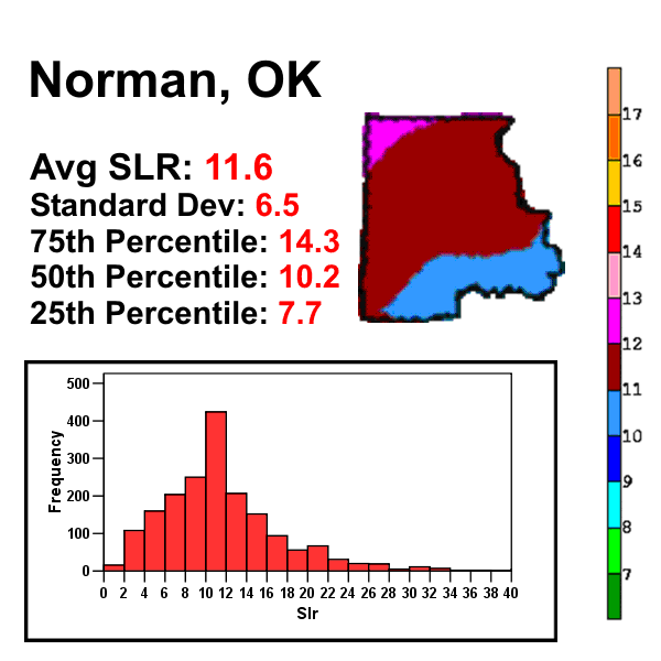
Instead of using the 2m temperature, perhaps the maximum temperature in the vertical profile (MaxTemp) may provide a more realistic snow ratio.  The snow ratio is inversely proportional to the MaxTemp.  The thinking behind the MaxTemp technique is that snow flakes entering into the warmest layer could be subjected to riming in which cloud liquid drops freeze directly onto the flakes helping to reduce interstitial spaces between ice and thereby increasing snow density and decreasing the snow to liquid ratio.  If we assume that MaxTemp is saturated then it seems reasonable that riming is more likely if MaxTemp is warmer because cloud liquid water content would also be higher. For this storm, the MaxTemp was forecasted to drop as the cold air deepened and thus the forecasted snow ratios for each SREF member increased with time.  The same SREF member we used above in figure 1 shows a lower snow ratio using the MaxTemp technique and the subsequent forecasted snowfall came out to nearly one foot, less than the 15" using the surface temperature. Even though the snow ratio is lower, it was still considerably higher than the mean snow ratio for central Oklahoma.

Figure 7  Like figure 6 except the snow accumulation and snow ratios are from the MaxTemp in profile snow ratio technique.  The yellow contours are temperature plotted as a function of time and height.

The next snow ratio technique, called the Zone Omega, evaluates the relationship between the vertical motion and temperature profile in the vertical.   In a brief explanation, the highest snow ratios occur when the greatest amount of lift occurs with the dendrite growth zone (-12 to -18 deg C) relative to the lift that occurs at warmer and colder temperatures. Likewise the highest snow ratios would occur if the vertical distribution of vertical motion falls outside the dendrite growth zone.  It so happens that the dendrite growth zone is the temperature layer in which cold phase precipitation production is most efficient, and that dendrites are prime candidate snow crystals to allow for the largest air spaces once dendrites aggregate.  So if the ascending air is focused in this layer, the predominant form of snow would be big fluffy, low density dendritic flakes (high snow ratio).  Vertical motion concentrated at lower levels (warmer temps) would yield snow flakes dominated by more compact needles at -5 deg C resulting in a lower snow ratio.  Likewise if the strongest vertical motion were concentrated at higher levels (lower temps) than the dendrite growth zone, then the predominate snow crystal habit would also be more compact plate, or column-shaped crystals resulting in a higher ratio. There is lots more discussion about this technique available at this address:  http://www.wdtb.noaa.gov/courses/winterawoc/IC6/lesson5/part1/player.html.  In addition, a Cobb and Waldstreicher (2005) is a good reference on this technique.

Considering the same SREF ARW WRF member as before, we find that the overall snowfall forecast decreased down to 9" in figure 8 when applying the Zone omega technique.  The snow ratio, in blue, was quite volatile as the level of peak ascent fell in and out of the dendrite growth zone (yellow contours).  Note that early on, the peak vertical motion was quite low resulting in a low snow ratio and then there was a relatively narrow window where the majority of ascent centered on the dendrite growth zone and the snow ratio spiked to 30:1 at 12-13 UTC on the 9th.  The greatest snowfall rate is more a function of the Zone Omega technique's huge snow ratios than the actual SWE rate visualized in figure 5. 

Figure 8  Similar to figure 6 except the Zone Omega technique is being used to calculate snow  fall.  In addition, instead of temperature, the contributing factors in the this technique include the vertical motion (red contours), and the dendrite growth zone (purple and yellow contours).  The yellow contours indicate when the dendrite growth zone is saturated. 

Just after the snow event ended around noon, I took a core sample of the snow using the standard 10" deep clearview rain gauge that is the standard for the COCORAHS observing network and melted it to get 0.37" of SWE.  Another similar gauge left open in the snow storm resulted in 0.41" of SWE.  Our SWE was below the featured SREF member (figures 5-8) but it was higher than the member with the minimum QPF.  So in short, our SWE was anticipated as a possibility according to the 21 UTC SREF model run.

Given a snow depth of only 2.7", my snow ratio was a paltry 6.6:1.  This value was well below even the most dense snow ratio technique applied above.  My snow ratio value was far below climatology as determined by Baxter et al. (2005) while the median value is near the median climatological value.  But all these values were well below the forecasted values by all SREF members, especially for those snow ratio techniques using temperature.  But even the Zone Omega technique overestimated the snow ratios during the forecasted maximum snowfall rates centered around 12 UTC.  But, earlier in the forecasted snowfall, the Zone Omega technique forecasted snow ratios < 10:1 when the maximum ascent didn't reach the dendrite production layer.

The measurements I mentioned so far represent the sum total of what happened in the storm.  But there's more complexity to the snow crystal types that yielded a broader variety of snow ratios.  I took a picture of our snow core balancing on the top of a ruler (official NWS ruler) and it showed some interesting changes in crystal types (fig. 9).  For instance, the lower third of the core consisted of tightly packed small crystals that appeared to be small graupel.  Above that layer, the middle third appeared to be small aggregates of small dendrites, still appearing quite dense.  Luckily, I measured the depth of these two layers before the third one fell in the late morning and got 2.2" of snow depth with 0.37" of SWE from the gauge and 0.31" from a core sample.  Just taking the 0.37" from the gauge, I got a snow ratio of only 5.9:1.  This layer of snow was dense, acting almost like machine-made snow but it was definitely not wet.  During the late morning, a final round of snow fell in the form of some of the biggest dendrites I've seen (see fig 10).  They were bundled up in large aggregates.  About 0.5" of snow accumulated with this last round and I got about .03 to .04" of SWE.  This ratio was a considerably larger 16:1, and quite expected for the flake type I saw. 

Figure 9  A picture of a snow core sample taken at 18 UTC 09 Feb 2011 showing a bottom layer of graupel, a middle layer of small dendrites and an upper layer of large dendrites.

Figure 10  A closeup picture of the upper layer of large dendrites that fell in the late morning of 09 Feb 2011 in east Norman.  Photo courtesy of Daphne LaDue.

Of all the snow ratio techniques that were used in this SREF model output, only the Zone Omega technique forecasted a similar broad range of values to what was observed.  Now, in the case of the Zone Omega technique, the forecast snow ratios were generally too high when the SWE rates were at their highest.  But at the start of the forecasted precipitation, the technique did forecast snow ratios less than 10:1 because the maximum ascent was expected to be centered well below the dendrite production zone.  Perhaps the technique represented some semblance of reality in central Oklahoma until the late morning when most of the snow ended. The morning sounding (fig. 10) from Norman during the first phase of the snow appears to support this idea since the cloud top may have barely risen into the heart of the dendrite production zone above 3 km MSL.   However the radar data showed a more complex picture.  The snow arrived in an almost convective band with reflectivities up to 30 dBZ at >5 km ARL around 1030 UTC.  This deep precipitation didn't last long so that by the time the sounding was launched at around 1115 UTC, the depth at maximum reflectivities fell to less than 3km ARL.   For most of the event, the observed snow production layer was quite shallow as observed by the KTLX radar.  Toward 16 UTC, the cooling aloft brought the dendrite production zone lower to phase with the layer of maximum ascent and as a result our last round of snow fell as low density dendrite aggregates.  The cold temperatures and weak ascent below this layer may have limited riming and additional higher density snow flake production.

figure 10.  A sounding display for Norman taken 09 Feb 2011, 12 UTC.

All of the snow ratio techniques that I discussed do little to consider the effects of solar radiation, temperature and wind upon the density of the snow pack.  I decided to measure the snow ratio after the end of the snow events, the first measurement coming at 13 UTC and the final one at 18 UTC after the large dendrites finished falling.  Temperatures near freezing could accelerate crystalline metamorphasis into denser forms and the snowpack density could increase.  There was some wind which could've broken the crystals upon landing and increased the density.  Roebber et al. (2003) described in detail these time dependent processes that alter the density of freshly fallen snow.  However, the temperatures for this event were less than 15 deg F and so I was not concerned about melting.  In addition, the snow core pictures didn't support the contention that the wind was strong enough to break a majority of crystals.   There was some natural settling to consider that may bring down the snow ratio forecasts a bit. BUFKIT attempts to account for settling by applying an exponential decay function to the forecast snow depth.  The effects of this function can be seen in figures 6-8.  Most of my measurement times were near the forecasted peak snowdepth and so this effect wasn't very significant.  


The Zone Omega technique may have won out in this case but I wouldn't vouche for its continued relative success for every event.  This technique doesn't account for errors in the vertical motion field, or other processes that include riming, and changes to snowpack density due to settling, wind, and melting.   In fact, for a well known New York City snowstorm on 26 January 2011 where 19" of snow fell in Central Park, the Zone Omega technique forecasted snow ratios that were far too high than observed.  In that case, relatively maximum elevated temperatures were closer to freezing and that layer featured a very strong flow ascending over the frontal surface ahead of strong low-level cyclogenesis.  In that case, the max temp in profile technique beat all others perhaps because that technique applies well when significant riming, and warm ice crystal production occurs in the face of strong saturated ascent at relatively warm temperatures.

Bottom line:

Our observed SWE was actually contained within the envelope of possible QPF based on the 21 UTC SREF.

The surface temperature and MaxTemp snow ratio techniques bombed terribly because the temperatures were cold.  Clearly these techniques failed to represent the mechanisms influencing the density of falling snow.  Dense snow can occur at very cold temperatures, surface or aloft.

The ZoneOmega technique performed the best of the three techniques but still far overestimated the snowfall.  Given the small snow ratios observed, and the compact crystal nature seen in the snow core, I suspect that much of the precipitation was forming below the dendrite production zone perhaps because the vertical motion field was too shallow.   Only when the temperatures cooled did the shallow vertical motion extend into the dendrite production zone.  Still, this technique did better than the others.  Don't expect this to be true all the time, however.

References

Baxter, A. A., C. E. Graves, J. T. Moore, 2005: A Climatology of Snow-to-Liquid Ratio for the Contiguous United States. Wea. Forecasting, 20, 729–744.  

Cobb, D. K., and J. Waldstreicher, 2005:  A simple physically-based snowfall algorithm.  Preprints, 21st Conf. on Weather Analysis and Forecasting, Washington D.C., American Meteorological Society

Roebber, P. J., S. L. Bruening, D. M. Schultz, J. V. Cortinas, 2003: Improving Snowfall Forecasting by Diagnosing Snow Density. Wea. Forecasting, 18, 264–287. 

2011-02-06 Freezing rain thunderstorms in Albany, NY

It's not often that thunder occurs in the northeast during the month of February.  When it does, there's probably only a few lightning strikes occuring over a relatively broad area.  Not this time.  Checking out the cloud-to-ground lightning maps in the area reveal lightning frequencies on par with some of the better summer-time convection in the same area.

Figure 1  Cloud to ground lightning map for the northeast US from 00 - 03 UTC.  The lightning strikes colored in white represent those within the first 12-30 minutes of this image time.  The yellow represents the 31-50 minute time frame.  Red indicates 51-70 minutes and so on.

 These thunderstorms formed as a line of ordinary cells aligned north-south axis.  The cells were more discrete in the southern portion of that line passing through western Massachusetts.  This radar capture below in figure 2 shows the cells as they passed just east of the Albany area.

figure 2

This kind of lightning frequency requires a substantial amount of instability.  Fortunately, the Albany sounding, launched just before 00Z provides an opportunity to sample the environment just ahead of the convection.  Indeed, the profile showed a region of strong elevated instability with steep lapse rates starting above the frontal surface at nearly 2 km AGL (see figure 3).

Figure 3.  A sounding from Albany, NY on 6 Feb 2011 00 UTC.

This convection fired up in the front end of a dry slot wrapping around the big upper-level wave to the north.  Such a configuration reminds me of a study by Carr and Millard (1985) where a dry slot aloft allows surface heating to commence while cooling continues aloft with unsaturated ascent ahead of the trough.  However, it's clear from the sounding that a saturated frontal inversion would prevent any surface heating from occurring in this event. 

Figure 4.  GOES12 IR image with cloud to ground lightning taken 6 Feb 2011, 0325 UTC.  Each color in the lightning represents 15 minute intervals.

So this event does have elements of dry slot convection and it also happens to fit a synoptic pattern in which the convection forms near or just north of the surface low as thundersnow events often do within the case selection process documented by Market et al. (2002).  Note the sea level pressure field in figure 5 relative to the active convection.

Figure 5.  Sea level pressure field relative to the composite reflectivity from the SPC mesoanalysis page. 

There is one major difference between this event and those studied by Market et al. (2002).  This event featured freezing rain.  But further north, the convection extended to a location where the sounding remained below freezing and snow could reach the ground.  Look at this RUC two hour forecast sounding in figure 6 from 02 UTC near Burlington, VT and the same midlevel instability appears there.

Figure 6.  The 00 UTC RUC 2 hour forecast valid 02 UTC 06 Feb 2011 for Burlington, VT.

Was this event forecasted?  Well, it was by some of the ensemble members in the SREF  model suite as you can see by this ensemble model sounding visualization in figure 7.

Figure 7.  Ensemble sounding display in BUFKIT from the 15 UTC 05 February 2011 9 hour forecast at Albany, NY.

Most of the permutations from the Regional Spectral Model showed significant instability in the midlevels.  Even though only 1/3 of the SREF members showed instability, that still amounts to a 30% chance of thunderstorms.  With the given hazards presented by these storms when considering the subfreezing lower atmospheric profile, it stands to good reason that identifying this thunderstorm potential ahead of time is a good idea.  This is especially true since the output in the SREF model agrees well with the synoptic patterns identified that commonly produce convection.  In fact, the SREF model output shown in concert with the pattern matching may help to overcome any inhibition for including thunderstorms in a forecast when it is climatologically and geographically rare.


Carr, Frederick H., James P. Millard, 1985: A Composite Study of Comma Clouds and their Association with Severe Weather over the Great Plains. Mon. Wea. Rev., 113, 370–387.

Market, Patrick S., Chris E. Halcomb, Rebecca L. Ebert, 2002: A Climatology of Thundersnow Events over the Contiguous United States. Wea. Forecasting, 17, 1290–1295.

Mountain sky and new snow over the BC coastal range

2010 December 28

We picked a fantastic day for skiing at Mt Seymour in the British Columbia coastal range after an overnight storm dropped some good winter snows down to a fairly low elevation.

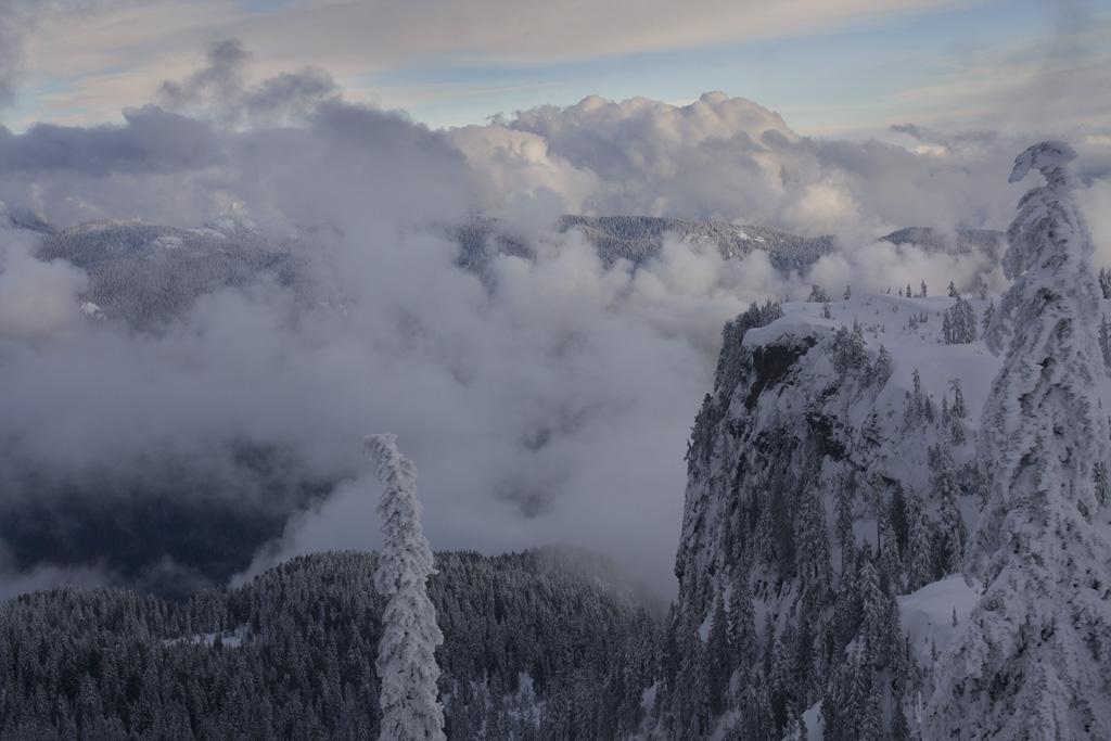
The storm left every tree on the mountain with low freezing levels but also low cloud base led to huge amounts of rime ice that added to the quality of the winter scene.   This entry is my attempt to explain the conditions that led to one of the prettier days on a mountain that I've had.  First, here are some shots.

This scene was taken at 2055 UTC from the top of Mt Seymour's highest lift facing west. 

 The trees were coated with fresh snow and rime from the previous evening.  Meanwhile, low-level moisture persisted behind the storm allowing low clouds to form on thermals helping to give the mountains an appearance of more height.  High clouds added depth to the sky.  In the case of the picture above, a large jet contrail appeared.  I'm typically not a fan of jet contrails but this one was interesting.  In fact a recent overpass from the MODIS Aqua polar orbiting satellite showed the same contrail about 40 minutes earlier.  See it below.

MODIS Aqua satellite full color visible image courtesy of MODIS today.

The blue triangle is the location of Mt. Seymour.

The low cloud cover increased just a bit to enhance the depth of the sky.  In some areas they provided a backdrop to further enhance the mountains.

An image facing west from the top of Mt. Seymour at 2255 UTC. 

 The mountain convection in nearly saturated air resulted in this updraft forming with a base below us and then flattening out on a stable layer above us.  This low cloud coverage was the maximum that we saw today.  Imagining what the sounding at our site looks like that would yield these clouds I took the Quillayute, WA, and the Kelowna, BC soundings and took my best guess as to what ours looked like.  See below.

The Quillayute, WA sounding in black is overlaid by teh Kelowna, BC sounding in orange.  My best guess sounding is in red.

I decided that the potential convective layer of the Quillayute sounding was a bit too shallow for us considering that I was already at 1300 m altitude and the cloud updraft ascended well above me.  However, the convective layer depth at Kelowna (100 mi northeast) implied a cold enough cloud tops for snow showers.  We saw no showers around the ski area.  So I believe the inversion where the clouds were flattening out was located higher than Quillayute but not by very much.  This picture below was to the east where similar shallow convection sets the backdrop of a spectacular valley.

The scene east of Mt. Seymour, BC taken 2309 UTC.

When the sun lowered further into the southwestern sky, the low clouds thinned out a little and the light warmed enough to allow me to take some shots across to Vancouver Island such as the one below. 

A view across the Salish sea toward Vancouver Island taken at 2329 UTC.

 Just after this shot, I noticed a peculiar cumulus cloud over over Burnaby well south of the terrain.  At first I didn't think much of it but after three chairlift rides up without seeing it dissipate, I figured there was a heat source that took advantage of the atmosphere that day to allow a semipersistent updraft to continue.  Perhaps there is a power plant underneath it somewhere.

A shot south of Mt. Seymour of a persistent cumulus cloud that may be partially anthropegenic in nature.  This shot was taken at 2353 UTC.

What made this day special was a combination of a relatively cold precipitation event the night before that dumped a fresh layer of new snow with added riming from a low cloud base and cold temperatures.  Then during the day, we had a shallow convective layer that allowed mountain cumulus to form but not so much as to flatten the lighting or obscure us in fog.  The high clouds were there to add depth but not so much to destroy the contrast.  I couldn't ask for a better setup considering the location.

I have more pictures at http://towerofstorms.net/gallery2/main.php?g2_itemId=4655