Extreme winds in California

One of the biggest southwestern US wind episodes in the last 10 years occurred on 01 to 02 December 2011 as an intense northerly pressure gradient formed between a near record strong surface high pressure system in the Pacific Northwest states and a relatively strong surface low formed in Arizona.  This wasn't any ordinary event.  Winds gusted to 92 mph in Pasadena - CA, 98 mph in Kane Springs - NV, 102 mph in Centerville - UT, 123 mph in Steamboat Springs - CO, and 150 mph at the top of Mammoth Mountain - CA!  There were winds to near hurricane force from central CA all the way east to western CO and south to near Albuquerque, NM.  Three selected maps show some of the other gusts around central CA (Figure 1), the Wasatch Valley (Figure 2), and the LA Basin (Figure 3).

Figure 1.  Peak wind gusts in mph for central CA on 01 December 2011.  (courtesy of  MesoWest)

Figure 2.  Peak wind gusts in mph for the Wasatch Valley, UT on 01 December 2011.  (courtesy of  MesoWest)

Figure 3.  Peak wind gusts in mph for the LA basin on 01 December 2011.  (courtesy of  MesoWest)

 Mammoth Mountain ski area on the eastern side of the central Sierra mountains certainly took top prize for the strongest wind gusts.  An anemometer recorded multiple peak gusts of 150 mph at the top of the gondola ride around 11 kft AGL(Figure 4)!  That so many wind gusts hit 150 mph means the anemometer may have proverbially 'hit the wall' and that the true wind may have been higher.  The worst of the winds occurred 00 - 06 PST (08 - 14 UTC) on 01 December.  

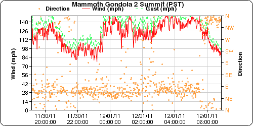Figure 4.  Wind meteogram of Gondola 2 summit anemometer on the top of Mammoth Mountain, CA.  (Courtesy of MesoWest)

These insane winds were primarily ridge top events that many other peaks all across the Sierras, Wasatch and numerous other mountains, likely shared.  But note that winds were much weaker just off the peaks.  As Figure 5 shows, other anemometers away from the ridges and peaks registered much lower winds.  An anemometer at the base of Mammoth only registered 5 mph!  What a difference a few feet makes!

Figure 5.  A micronet plot of stations on Mammoth Mountain, CA at 01 December 2011 - 05 UTC.

Needless to say this intense wind event resulted in numerous reports of damage.  There are too many to list here but the highlights include 400 buildings damaged in Pasadena with 40 of those evacuated, a roof blown off a condo in Steamboat Springs - CO, and multiple trucks blown off I-15 north of Salt Lake City.  The Capital Weather Gang provided a wealth of information, pictures and video regarding the impacts of this event in one of their posts.

What caused this event to be so intense?  There was a big upper-level trough diving southward with very strong winds on its west side (Figure 6).  This amplification set the stage to intensify the low-level low over western Arizona while at the same time a strong low-level high built into the Pacific Northwest.  The increase in the pressure gradient between these two features helped to rapidly enhance the northeasterly winds.  This setup is common in the Southwest US leading to the infamous Santa Ana Winds.  During a typical cool season, the LA Basin can expect 20 of these events based on a study by Raphael (2003).  This one, however, was exceptionally strong.  But how strong was it in compared to the climatology?

Figure 6.  500 mb heights and observations for 01 December 2011 00 UTC ( top left) and 12 UTC (top right).  850 mb heights and observations for the same date 00 UTC (bottom left) and 12 UTC (bottom right).  Courtesy of SPC.

One way to compare to a climatology is to look at how the sea-level pressure pattern of this event matches that of other Santa Ana events.  In figure 7, the sea level pressure analysis from the Short Range Ensemble Forecast System showed a 1000 mb low in Arizona and a 1040 mb ridge from Washington state to Montana.  A composite of Santa Ana events compiled by Jones et al. (2010) only yields a 1028 mb sea-level high in Wyoming and a 1016 mb low just south of Arizona.  Clearly this event exhibited a much stronger pressure gradient than the composite.  However you could argue composites appear weak just by the way they average out the placement of individual low and high centers.  

Another way to compare with climatology is through standardized anomalies in a similar manner to Hart and Grumm (2001).  Without going into a long description of using standardized anomalies, they infer how many standard deviations from the mean a particular parameter happens to be.  For sea-level pressure, standardized anomalies reached -3 standard deviations for the sea-level low at 09 UTC on 01 December while the corresponding high reached 2 standard deviations for the same time (Figure 7).  These values persisted for several hours during the morning before the low filled slightly during the late afternoon.  It certainly represented a stronger than normal Santa Ana sea-level pressure pattern but there have been stronger sea level pressure standardized anomalies from non Santa Ana events.    

The mean height standardized anomalies for multiple pressure levels up to 250 mb at 09 UTC (Mheight) also do not show any standout values (< +- 4), especially considering that the top 10 events of Mheight all had values greater than 5 (see Graham and Grumm 2010).  

However the standardized anomalies for wind painted a much stronger event.  Low-level standardized anomalies were analyzed by the SREF to exceed +- 5 standard deviations for both the U and V components, especially over southern CA and along the Wasatch mountains (Figure 7).  The 15 UTC analysis showed values exceeding 6 standard deviations in northern UT!  Considering that the analysis in Figure 7 represents the mean of 21 members, these numbers are quite impressive.  The anomalies drop off with height so that at 250 mb, we only see 3-4 standard deviations along the back side of the trough.  Now I don't have all the standardized anomalies for wind for each pressure level but I say that there is a possibility for these wind anomalies to reach the top 20 and maybe the top 10 events in the western US for wind as determined by Mwind found by Graham and Grumm (2010).  Mwind is the mean of the maximum absolute standardized anomalies found for each pressure level across the western US.  The Mwind ranges from 4.5 to 4.9 for the top 10 events using Mwind.  So now we're seeing the possibility that this wind event is not only the worst Santa Ana event in 10 years for southern CA but may rank among the 10 biggest events for the western US.  Remember this event was widespread across a huge chunk of real-estate.

Figure 7.  The output from the  01 December 2011 - 09 UTC short range ensemble forecasting system output including sea level pressure contours with standardized anomalies (shaded, upper left), and 850 mb winds with V (U) wind standardized anomalies in the lower left (lower right) panels.  The upper right panel shows a composite sea level pressure pattern for Santa Ana wind events for 20 years ending in 2008 from Jones et al. (2010).

The standardized anomalies can be used to also show how rare some of these events happen to be.  If measured by sea-level pressure, the return period for the maximum value found (negative 3-4 standard deviations) would only be once every few months (Figure 8).    However, we don't have a calculation of return intervals of the difference between the maximum and minimum standardized anomaly in the Western US.  Had we such information, we may find a much longer return interval.  This chart can be found in the Western Region standardized anomaly webpage.

Figure 8.  Sea level pressure standardized anomaly return periods for the western half of the U.S. based on the North American Regional Reanalysis data (from Graham and Grumm, 2010). The red vertical lines represent the maximum and minimum standardized anomalies for 01 December 2011 in the same area.

The standardized anomaly return periods for winds at 850 mb does show a much longer return period for both the U and V components.  In fact, judging by the noisy trends at the +- 5 standard deviations range, there have not been too many events to construct a reliable return interval.  What we do see is a value in excess of 100 months or close to 10 years.  Wait, the media's claiming the Santa Ana event was also the worst in 10 years!  Is this coincidence by design?  Well, not likely and more likely this is coincidence.

Figure 9.  Similar to figure 8 except for  850 mb V-wind (U wind) standardized anomalies in the top (bottom) panels respectively.

The synoptics showed the case for a widespread wind event.  The details are very much governed by local topography.  Given the variety of the topography in the west, we could expect to see a wide variety of behavior in the localized enhanced wind.

As an example,  there is the ridge top wind to consider and the SierraNevada mountains are well known for this phenomenon.  To highlight the Mammoth Mountain extreme winds, let's take a look at the    10 hour forecast sounding profile from the NAM (Figure 10) taken from near Bridgeport lake, CA.  This sounding site is located about 30 mi north of Mammoth Mountain ski area.  The winds were unusual in the combination of the strength and direction.  Almost the full component of the wind was normal to the orientation of the Sierras and a rule of thumb that the NWS office in Reno used in their ridge-top wind forecasts was to double the ridge-level  winds.  A doubling of the winds resulted in a forecasted 110 mph sustained winds at the top of Mammoth Mountain by 10 UTC.  That's a little short of the observations as winds were hitting a sustained 140 mph well before this time.

The time-height forecast for this site showed that the winds at 1 km (AGL) were strengthening all the way to 15 UTC (Figure 11).  However the strongest observed winds plateaued starting at 07 UTC. It's possible that the ridge top stable layer helped promote an acceleration of the winds helping to accelerate them more than the rule of thumb.   Assuming the relationship continued as the forecasted winds increased to 80 kts, then I can understand concerns by forecasters of wind gusts reaching 200 mph at mountain top by 15 UTC.  Hindsight revealed that the strongest winds occurred around 07-09 UTC.  We'll never know how strong they were because the anemometer's maximum possible reading appeared to be 150 mph.

 

Figure 10.  A WDTB WRF ensemble 10 hour forecast sounding from the NAM NMM 212 KF member valid 01 December  2011 - 10 UTC for a site KBDG near Mammoth Mountain, CA.  The hodograph range rings are in 10 m/s intervals and the white diagonal represents the axis of the SierraNevada mountains.  The wind profile is marked by the yellow line segments from the surface to 6 km AGL.  On the SKEWT, the shaded brown region in the lowest km represents the height of Mammoth Mountain with respect to the altitude of KBDG.  More information on the rest of the display can be found in the WDTB BUFKIT webpage.

Figure 11. A time-height plot of the same forecast model, location, and time as in Figure 10.  The contours show forecast horizontal wind in kts.  The brown shaded region indicates the height of Mammoth Mountain from KBDG.  

Whereas the Sierra ridge top case showed an example of Bernoulli acceleration with possible enhancement by an appropriately positioned stable layer, the Santa Ana local wind appeared to be induced by a mountain wave.  From the same model run, we took a 7 hour forecast from the 01 December - 00 UTC run for Ontario, CA (Figure 12).  Here, there's more evidence that a critical layer may have helped to trap lee waves.  While the component of the winds perpendicular to the San Bernardino mountains never was forecast to reach zero, there was a forecasted reversal in shear close to ridge top level.  There was also a stable layer forecasted to be located near the ridge top too.  Now the morning soundings didn't show the stable layer as pronounced as forecast at ridge top but the reversal of shear was observed at San Diego.  Perhaps somewhere a critical layer did form exacerbating a downslope wind event.  Perhaps that location happened to be Pasadena where widespread damage was observed.  Too bad there weren't any observed soundings in the area the morning of 01 December.

Figure 12.  Similar to Figure 10 except for Ontario, CA valid at 07 UTC .

References:

Graham, R.A., R. H. Grumm, 2010: Utilizing Normalized Anomalies to Assess Synoptic-Scale Weather Events in the Western United States. Wea. Forecasting, 25, 428–445.

Hart, R., and R. H. Grumm, 2001: Using normalized climatological anomalies to rank synoptic-scale events objectively. Mon. Wea. Rev., 129, 2426–2442.

Jones, C., F. Fujioka, L. M. V. Carvalho, 2010: Forecast Skill of Synoptic Conditions Associated with Santa Ana Winds in Southern California. Mon. Wea. Rev., 138, 4528–4541.

Raphael, M. N., 2003: The Santa Ana Winds of California. Earth Interact., 7, 1–13.